Human-Like Machine Hearing With AI (1/3)

Applying neural networks in real-time audio signal processing

Significant breakthroughs in AI technology have been achieved through modeling human systems. While artificial neural networks (NNs) are mathematical models which are only loosely coupled with the way actual human neurons function, their application in solving complex and ambiguous real-world problems has been profound. Additionally, modeling the architectural depth of the brain in NNs has opened up broad possibilities in learning more meaningful representations of data.

If you’ve missed out on the other articles, click below to get up to speed:

Background: The promise of AI in audio processing
Criticism: What’s wrong with CNNs and spectrograms for audio processing?
Part 2: Human-Like Machine Hearing With AI (2/3)

In image recognition and processing, the inspiration from the complex and more spatially invariant cells of the visual system in CNNs has also produced great improvements to our technologies. If you’re interested in applying image recognition technologies on audio spectrograms, check out my article “What’s wrong with CNNs and spectrograms for audio processing?”.

As long as human perceptual capacity exceeds that of machines, we stand to gain by understanding the principles of human systems. Humans are very skillful when it comes to perceptual tasks and the contrast between human understanding and the status quo of AI becomes particularly apparent in the area of machine hearing. Considering the benefits reaped from getting inspired by human systems in visual processing, I propose that we stand to gain from a similar process in machine hearing with neural networks.

In this article series, I will detail a framework for real-time audio signal processing with AI which was developed in cooperation with Aarhus University and intelligent loudspeaker manufacturer Dynaudio A/S. Its inspiration is primarily drawn from cognitive science which attempts to combine perspectives of biology, neuroscience, psychology and philosophy to gain greater understanding of our cognitive faculties.

Cognitive Sound Properties

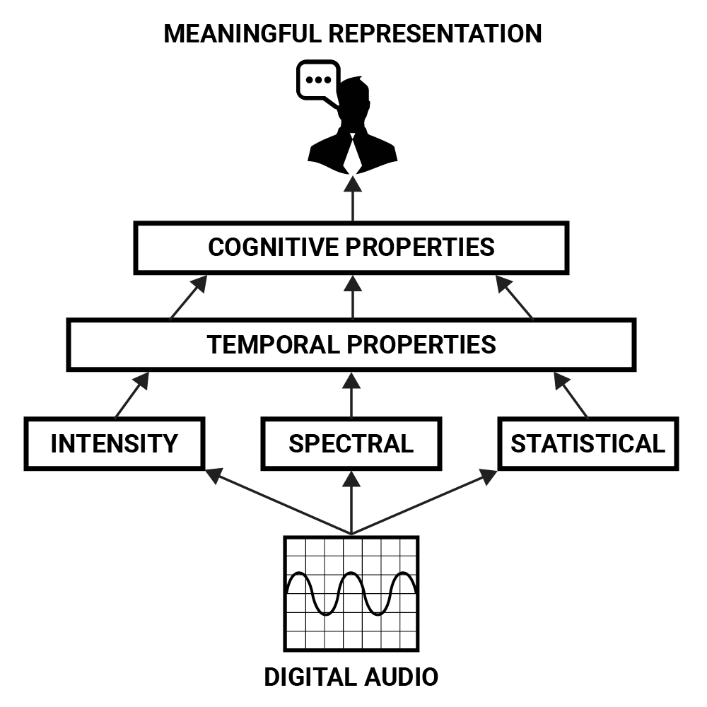
Perhaps the most abstract domain of sound is how we, as humans, perceive it. While a solution for a signal processing problem has to operate within the parameters of intensity, spectral and temporal properties on a low level, the end goal is most often a cognitive one: Transforming a signal in such a way that our perceptions of the sounds it contains are altered.

If one wishes to programatically change the gender of a recorded spoken voice for example, it is necessary to describe this problem in more meaningful terms before defining its lower level characteristics. The gender of a speaker can be conceived as a cognitive property which is constructed from many factors: General pitch and timbre of a voice, differences in pronunciation, differences in choice of words and language and a common understanding of how these properties relate to gender.

These parameters can be described in lower level features like intensity, spectral and temporal properties but only in more complex combinations do they form high-level representations. This forms a hierarchy of audio features from which the “meaning” of a sound can be derived. The cognitive property representing a human voice can be thought of as a combinatory pattern of temporal developments in a sound’s intensity, spectral and statistical properties.

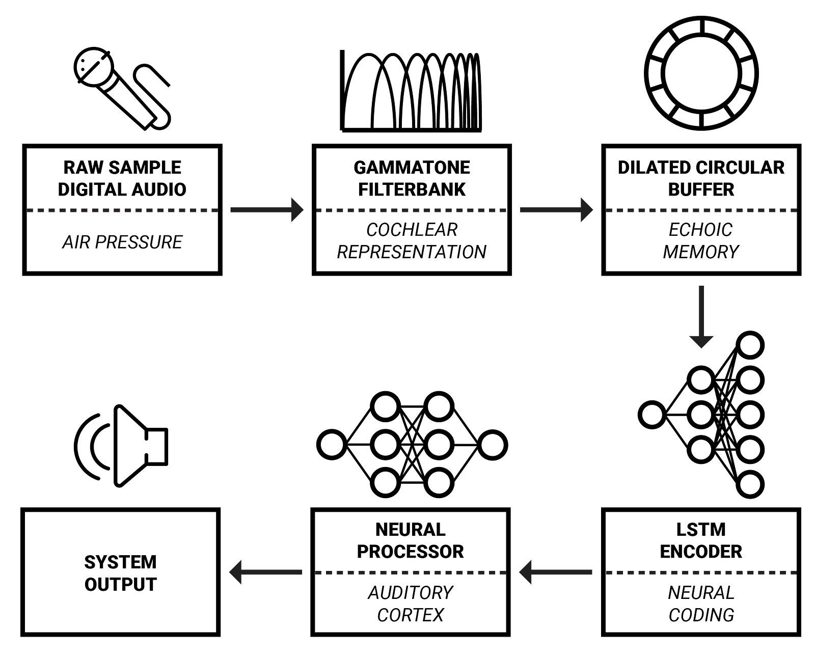
NNs are great at extracting abstracted representations of data and are therefore well suited for the task of detecting cognitive properties in sound. In order to build a system for this purpose, let’s examine how sound is represented in human auditory organs that we can use to inspire representation of sound for processing with NNs.

Cochlear Representation

Hearing in humans starts at the outer ear which firstly consists of the pinna. The pinna acts as a form of spectral preprocessing in which the incoming sound is modified depending on its direction in relation to the listener. Sound then travels through the opening in the pinna into the ear canal which further acts to modify spectral properties of incoming sound by resonating in a way that amplifies frequencies in the range ~1–6 kHz [1].

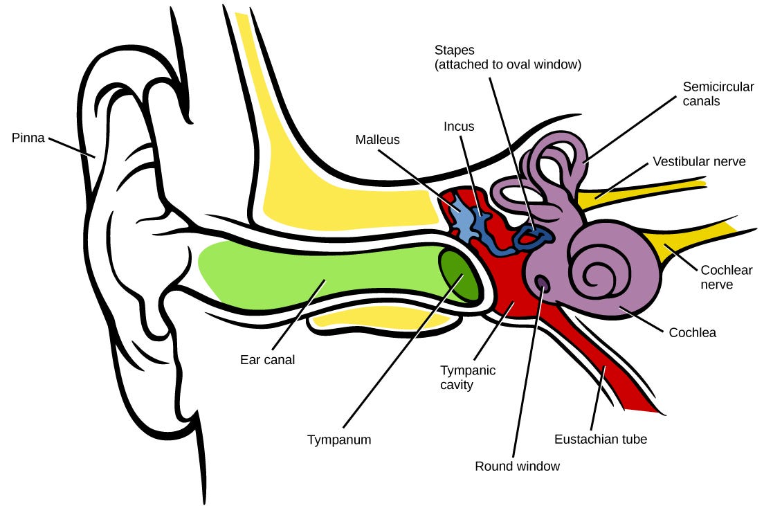
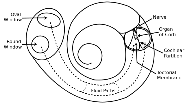
As sound waves reach the end of the ear canal, they excite the eardrum onto which the ossicles (the smallest bones in the body) are attached. These bones transmit the pressure from the ear canal to the fluid-filled cochlea in the inner ear [1]. The cochlea is of great interest in guiding sound representation for NNs because this is the organ responsible for transducing acoustic vibrations into neural activity in humans .

It is a coiled tube which is separated along its length by two membranes being the Reissner’s membrane and the basilar membrane. Along the length of the cochlea, there is a row of around 3,500 inner hair cells [1]. As pressures enter the cochlea, its two membranes are pushed down. The basilar membrane is narrow and stiff at its base but loose and wide at its apex so that each place along its length responds more intensely at a particular frequency.

To simplify, the basilar membrane can be thought of as a continuous array of bandpass filters which, along the length of the membrane, acts to separate sounds into their spectral components.

This is the primary mechanism by which humans convert sound pressures into neural activity. Therefore, it is reasonable to assume that spectral representations of audio would be beneficial in modeling sound perception with AI. Since frequency responses along the basilar membrane vary exponentially [2], logarithmic frequency representations might prove most efficient. One such representation could be derived using a gammatone filterbank. These filters are commonly applied in modeling spectral filtering in the auditory system since they approximate the impulse response of human auditory filters derived from the measured auditory nerve fiber response to white noise stimuli called the “revcor” function [3].

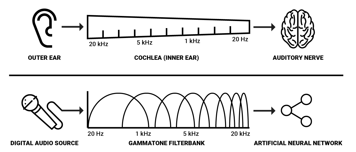
Since the cochlea has ~3500 inner hair cells and humans can detect gaps in sounds down to ~2–5 ms in length [1], a spectral resolution of 3500 gammatone filters separated into 2 ms windows seem optimal parameters for achieving human-like spectral representation in machines. In practical scenarios however, I assume that lesser resolutions could still achieve desirable effects in most analysis and processing tasks while being more viable from a computational standpoint.

A number of software libraries for auditory analysis are available online. A notable example is the Gammatone Filterbank Toolkit by Jason Heeris. It provides adjustable filters as well as tools for spectrogram-like analysis of audio signals with gammatone filters.

Neural Coding

As neural activity moves from the cochlea onto the auditory nerve and the ascending auditory pathways, a number of processes are applied in brainstem nuclei before it reaches the auditory cortex.

These processes form a neural code which represents an interface between stimulus and perception [4]. Much knowledge about the specific inner workings of these nuclei is still speculative or unknown, so I will detail these nuclei only at their higher levels of functioning.

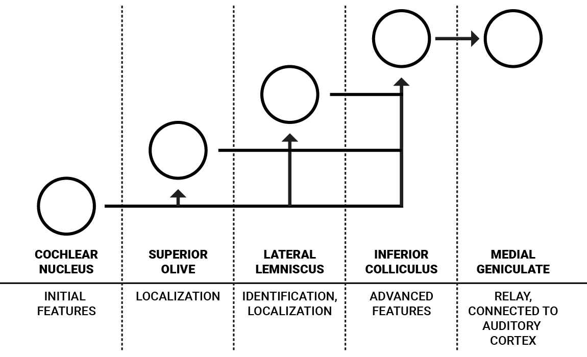
Humans have a set of these nuclei for each ear that are interconnected, but for simplicity, I’ve illustrated the flow for only one ear. The cochlear nucleus is the first coding step for neural signals coming from the auditory nerve. It consists of a variety of neurons with different properties which serve to perform initial processing of sound features, some of which are directed to the superior olive which is associated with sound localization while others are directed to the lateral lemniscus and inferior colliculus, commonly associated with more advanced features [1].

J. J. Eggermont details this flow of information from the cochlear nucleus in “Between sound and perception: reviewing the search for a neural code” as follows: “The ventral [cochlear nucleus] (VCN) extracts and enhances the frequency and timing information that is multiplexed in the firing patterns of the [auditory nerve] fibers, and distributes the results via two main pathways: the sound localization path and the sound identification path. The anterior part of the VCN (AVCN) mainly serves the sound localization aspects and its two types of bushy cells provide input to the superior olivary complex (SOC), where interaural time differences (ITDs) and level differences (ILDs) are mapped for each frequency separately” [4].

The information carried by the sound identification pathway is a representation of complex spectra such as vowels. This representation is mainly created in the ventral cochlear nucleus by special types of units dubbed “chopper” (stellate) neurons [4]. The details of these auditory encodings are difficult to specify but they indicate to us that a form of “coding” of incoming frequency spectra could improve understanding of low level sound features as well as making sound impressions less expensive to process in NNs.

Spectral Sound Embeddings

We can apply the unsupervised autoencoder NN architecture as an attempt to learn common properties associated with complex spectra. Like word embeddings, its possible to find commonalities in frequency spectra that represent select features (or a more tightly condensed meaning) of sounds.

An autoencoder is trained to encode an input into a compressed representation that can be reconstructed back into a representation with a high similarity to the input. This means that the autoencoder’s target output is the input itself [5]. If an input can be reconstructed without great loss, the network has learnt to encode it in such a way that the compressed internal representation contains enough meaningful information. This internal representation is then what we refer to as the embedding. The encoding part of the autoencoder can be decoupled from the decoder to generate embeddings for other applications.

Embeddings also have the benefit that they are often of lower dimensionality than the original data. For instance, an autoencoder could compress a frequency spectrum with a total of 3500 values into a vector with a length of 500 values. Put simply, each value of such a vector could describe higher level factors of a spectrum such as vowel, harshness or harmonicity - These are only examples, as the meaning of statistically common factors derived by an autoencoder might often be difficult to label in plain language.

In the next article, we will expand upon this idea with added memory to produce embeddings for temporal developments of audio frequency spectra.

References

[1] C. J. Plack, The Sense of Hearing, 2nd ed. Psychology Press, 2014.
[2] S. J. Elliott and C. A. Shera, “The cochlea as a smart structure,” Smart Mater. Struct., vol. 21, no. 6, p. 64001, Jun. 2012.
[3] A.M. Darling, “Properties and implementation of the gammatone filter: A tutorial”, Speech hearing and language, University College London, 1991.
[4] J. J. Eggermont, “Between sound and perception: reviewing the search for a neural code.,” Hear. Res., vol. 157, no. 1–2, pp. 1–42, Jul. 2001.
[5] T. P. Lillicrap et al., Learning Deep Architectures for AI, vol. 2, no. 1. 2015.