


DISCLAIMER: This article was migrated from the legacy personal technical blog originally hosted here, and thus may contain formatting and content differences compared to the original post. Additionally, it likely contains technical inaccuracies, opinions that the author may no longer align with, and most certainly poor use of English. This article remains public for those who may find it useful despite its flaws.
Gaussian blur is an image space effect that is used to create a softly blurred version of the original image. This image then can be used by more sophisticated algorithms to produce effects like bloom, depth-of-field, heat haze or fuzzy glass. In this article I will present how to take advantage of the various properties of the Gaussian filter to create an efficient implementation as well as a technique that can greatly improve the performance of a naive Gaussian blur filter implementation by taking advantage of bilinear texture filtering to reduce the number of necessary texture lookups. While the article focuses on the Gaussian blur filter, most of the principles presented are valid for most convolution filters used in real-time graphics.
Gaussian blur is a widely used technique in the domain of computer graphics and many rendering techniques rely on it in order to produce convincing photorealistic effects, no matter if we talk about an offline renderer or a game engine. Since the advent of configurable fragment processing through texture combiners and then using fragment shaders the use of Gaussian blur or some other blur filter is almost a must for every rendering engine. While the basic convolution filter algorithm is a rather expensive one, there are a lot of neat techniques that can drastically reduce the computational cost of it, making it available for real-time rendering even on pretty outdated hardware. This article will be most like a tutorial article that tries to present most of the available optimization techniques. Some of them may be familiar to all of you but maybe the linear sampling will bring you some surprise, but let’s not go that far but start with the basics.
Terminology
In order to precede any possibility of confusion, I’ll start the article with the introduction of some terms and concepts that I will use in the post.
Convolution filter – An algorithm that combines the color value of a group of pixels.
NxN-tap filter – A filter that uses a square shaped footprint of pixels with the square’s side length being N pixels.
N-tap filter – A filter that uses an N-pixel footprint. Note that an N-tap filter does *not* necessarily mean that the filter has to sample N texels as we will see that an N-tap filter can be implemented using less than N texel fetches.
Filter kernel – A collection of relative coordinates and weights that are used to combine the pixel footprint of the filter.
Discrete sampling – Texture sampling method when we fetch the data of exactly one texel (aka GL_NEAREST filtering).
Linear sampling – Texture sampling method when we fetch a footprint of 2×2 texels and we apply a bilinear filter to aquire the final color information (aka GL_LINEAR filtering).
Gaussian filter
The image space Gaussian filter is an NxN-tap convolution filter that weights the pixels inside of its footprint based on the Gaussian function:

The pixels of the filter footprint are weighted using the values got from the Gaussian function thus providing a blur effect. The spacial representation of the Gaussian filter, sometimes referred to as the “bell surface”, demonstrates how much the individual pixels of the footprint contribute to the final pixel color.

Based on this some of you may already say “aha, so we simply need to do NxN texture fetches and weight them together and voilà”. While this is true, it is not that efficient as it looks like. In case of a 1024×1024 image, using a fragment shader that implements a 33×33-tap Gaussian filter based on this approach would need an enormous number of 1024*1024*33*33 ≈ 1.14 billion texture fetches in order to apply the blur filter for the whole image.
In order to get to a more efficient algorithm we have to analyze a bit some of the nice properties of the Gaussian function:
- The 2-dimensional Gaussian blur can be applied by combining two 1-dimensional Gaussian blurs:

- Applying successive Gaussian blurs has the same effect as applying a single, larger Gaussian blur, whose radius is the square root of the sum of the squares of the blur radii.
Both of these properties of the Gaussian function give us room for optimization opportunities.
Based on the first property, we can separate our 2-dimensional Gaussian function into two 1-dimensional one. In case of the fragment shader implementation this means that we can separate our Gaussian filter into a horizontal blur filter and the vertical blur filter, still getting the accurate results after the rendering. This results in two N-tap filters and an additional rendering pass needed for the second filter. Getting back to our example, applying the two filters to a 1024×1024 image using two 33-tap Gaussian filters will get us to 1024*1024*33*2 ≈ 69 million texture fetches. That is more than an order of magnitude less than the original approach made possible.
The second property can be used to bypass hardware limitations on platforms that support only a limited number of texture fetches in a single pass.
Gaussian kernel weights
We’ve seen how to implement an efficient Gaussian blur filter for our application, at least in theory, but we haven’t talked about how we should calculate the weights for each pixel we combine using the filter in order to get the proper results. The most straightforward way to determine the kernel weights is by simply calculating the value of the Gaussian function for various distribution and coordinate values. While this is the most generic solution, there is a simpler way to get some weights by using the binomial coefficients. Why we can do that? Because the Gaussian function is actually the distribution function of the normal distribution and the normal distribution’s discrete equivalent is the binomial distribution which uses the binomial coefficients for weighting its samples.
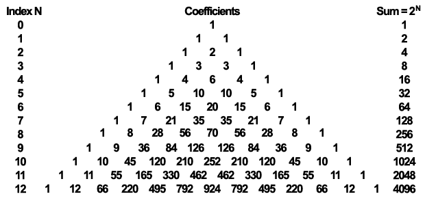
For implementing our 9-tap horizontal and vertical Gaussian filter we will use the last row of the Pascal triangle illustrated above in order to calculate our weights. One may ask why we don’t use the row with index 8 as it has 9 coefficients. This is a justifiable question, but it is rather easy to answer it. This is because with a typical 32 bit color buffer the outermost coefficients don’t have any effect on the final image while the second outermost ones have little to no effect. We would like to minimize the number of texture fetches but provide the highest quality blur as possible with our 9-tap filter. Obviously, in case very high precision results are a must and a higher precision color buffer is available, preferably a floating point one, using the row with index 8 is better. But let’s stick to our original idea and use the last row…
By having the necessary coefficients, it is very easy to calculate the weights that will be used to linearly interpolate our pixels. We just have to divide the coefficient by the sum of the coefficients that is 4096 in this case. Of course, for correcting the elimination of the four outermost coefficients, we shall reduce the sum to 4070, otherwise if we apply the filter several times the image may get darker.
Now, as we have our weights it is very straightforward to implement our fragment shaders. Let’s see how the vertical file shader will look like in GLSL:
uniform sampler2D image;

out vec4 FragmentColor;

uniform float offset[5] = float[](0.0, 1.0, 2.0, 3.0, 4.0);
uniform float weight[5] = float[](0.2270270270, 0.1945945946, 0.1216216216,
                                  0.0540540541, 0.0162162162);

void main(void) {

    FragmentColor = texture2D(image, vec2(gl_FragCoord) / 1024.0) * weight[0];

    for (int i=1; i<5; i++) {

        FragmentColor +=
            texture2D(image, (vec2(gl_FragCoord) + vec2(0.0, offset[i])) / 1024.0)
                * weight[i];

        FragmentColor +=
            texture2D(image, (vec2(gl_FragCoord) - vec2(0.0, offset[i])) / 1024.0)
                * weight[i];
    }
}
Obviously the horizontal filter is no different just the offset value is applied to the X component rather than to the Y component of the fragment coordinate. Note that we hardcoded here the size of the image as we divide the resulting window space coordinate by 1024. In a real life scenario one may replace that with a uniform or simply use texture rectangles that don’t use normalized texture coordinates.
If you have to apply the filter several times in order to get a more strong blur effect, the only thing you have to do is ping-pong between two framebuffers and apply the shaders to the result of the previous step.

Linear sampling
So far, we were able to see how to implement a separable Gaussian filter using two rendering pass in order to get a 9-tap Gaussian blur. We’ve also seen that we can run this filter three times over a 1024×1024 sized image in order to get a 33-tap Gaussian blur by using only 56 million texture fetches. While this is already quite efficient it does not really expose any possibilities of the GPUs as this form of the algorithm would work perfectly almost unmodified on a CPU as well.
Now, we will see that we can take advantage of the fixed function hardware available on the GPU that can even further reduce the number of required texture fetches. In order to get to this optimization let’s discuss one of the assumptions that we made from the beginning of the article:
So far, we assumed that in order to get information about a single pixel we have to make a texture fetch, that means for 9 pixels we need 9 texture fetches. While this is true in case of a CPU implementation, it is not necessarily true in case of a GPU implementation. This is because in the GPU case we have bilinear texture filtering at our disposal that comes with practically no cost. That means if we don’t fetch at texel center positions our texture then we can get information about multiple pixels. As we already use the separability property of the Gaussian function we actually working in 1D so for us bilinear filter will provide information about two pixels. The amount of how much each texel contribute to the final color value is based on the coordinate that we use.
By properly adjusting the texture coordinate offsets we can get the accurate information of two texels or pixels using a single texture fetch. That means for implementing a 9-tap horizontal/vertical Gaussian filter we need only 5 texture fetches. In general, for an N-tap filter we need [N/2] texture fetches.
What this will mean for our weight values previously used for the discrete sampled Gaussian filter? It means that each case we use a single texture fetch to get information about two texels we have to weight the color value retrieved by the sum of the weights corresponding to the two texels. Now that we know what are our weights, we just have to calculate the texture coordinate offsets properly.
For texture coordinates, we can simply use the middle coordinate between the two texel centers. While this is a good approximation, we won’t accept it as we can calculate much better coordinates that will result us exactly the same values as when we used discrete sampling.
In case of such a merge of two texels we have to adjust the coordinates that the distance of the determined coordinate from the texel #1 center should be equal to the weight of texel #2 divided by the sum of the two weights. In the same style, the distance of the determined coordinate from the texel #2 center should be equal to the weight of texel #1 divided by the sum of the two weights.
As a result, we get the following formulas to determine the weights and offsets for our linear sampled Gaussian blur filter:

By using this information we just have to replace our uniform constants and decrease the number of iterations in our vertical filter shader and we get the following:
uniform sampler2D image;

out vec4 FragmentColor;

uniform float offset[3] = float[](0.0, 1.3846153846, 3.2307692308);
uniform float weight[3] = float[](0.2270270270, 0.3162162162, 0.0702702703);

void main(void) {

    FragmentColor = texture2D(image, vec2(gl_FragCoord) / 1024.0) * weight[0];

    for (int i=1; i<3; i++) {

        FragmentColor +=
            texture2D(image, (vec2(gl_FragCoord) + vec2(0.0, offset[i])) / 1024.0)
                * weight[i];

        FragmentColor +=
            texture2D(image, (vec2(gl_FragCoord) - vec2(0.0, offset[i])) / 1024.0)
                * weight[i];
    }
}
This simplification of the algorithm is mathematically correct and if we don’t consider possible rounding errors resulting from the hardware implementation of the bilinear filter we should get the exact same result with our linear sampling shader like in case of the discrete sampling one.

While the implementation of the linear sampling is pretty straightforward, it has a quite visible effect on the performance of the Gaussian blur filter. Taking into consideration that we managed to implement a 9-tap filter using just five texture fetches instead of nine, back to our example, blurring a 1024×1024 image with a 33-tap filter takes only 1024*1024*5*3*2 ≈ 31 million texture fetches instead of the 56 million required by discrete sampling. This is a quite reasonable difference and in order to better present how much that matters I’ve done some experiment to measure the difference between the two techniques. The result speaks for itself:

As we can see, the performance of the Gaussian filter implemented with linear sampling is about 60% faster than the one implemented with discrete sampling indifferent from the number of blur steps applied to the image. This roughly proportional to the number of texture fetches spared by using linear filtering.
Conclusion
We’ve seen that implementing an efficient Gaussian blur filter is quite straightforward and the result is a very fast real-time algorithm, especially using the linear sampling, that can be used as the basis of more advanced rendering techniques.
Even though we concentrated on Gaussian blur in this article, many of the discussed principles apply to most convolution filter types. Also, most of the theory applies in case we need a blurred image of reduced size like it is usually needed by the bloom effect, even the linear sampling. The only thing that is really different in case of a reduced size blurred image is that our center pixel is also a “double-pixel”. This means that we have to use a row from our Pascal triangle that has even number of coefficients as we would like to linear sample the middle texels as well.
We’ve also had a brief insight into the computational complexity of the various techniques and how the filter can be efficiently implemented on the GPU.
The demo application used for the measurements performed to compare the discrete and linear sampling method can be downloaded here:
Links: source code, Win32 binary